Ultimate Guide To Text Similarity With Python

In this article, you will learn about different similarity metrics and text embedding techniques. By the end, you'll have a good grasp of when to use what metrics and embedding techniques. You’ll also get to play around with them to help establish a general intuition.

You can find the accompanying web app here.

Topics Covered In This Article

• Text Similarity - Jaccard, Euclidean, Cosine
• Text Embeddings
• Word Embeddings
•     One-Hot Encoding & Bag-of-Words
•     Term Frequency-Inverse Document Frequency (TF-IDF)
•     Word2Vec
• Embeddings from Language Models
• Sentence Embeddings: Doc2Vec
• Sentence Transformers
• Universal Sentence Encoder

Understanding Similarity

Similarity is the distance between two vectors where the vector dimensions represent the features of two objects. In simple terms, similarity is the measure of how different or alike two data objects are. If the distance is small, the objects are said to have a high degree of similarity and vice versa. Generally, it is measured in the range 0 to 1. This score in the range of [0, 1] is called the similarity score.

An important point to remember about similarity is that it’s subjective and highly dependent on the domain and use case. For example, two cars can be similar because of simple things like the manufacturing company, color, price range, or technical details like fuel type, wheelbase, horsepower. So, special care should be taken when calculating similarity across features that are unrelated to each other or not relevant to the problem.

As simple as the idea may be, similarity forms the basis of many machine learning techniques. For instance, the K-Nearest-Neighbors classifier uses similarity to classify new data objects, similarly, K-means clustering utilizes similarity measures to assign data points to appropriate clusters. Even recommendation engines use neighborhood-based collaborative filtering methods which use similarity to identify a user’s neighbors.

The use of similarity measures is quite prominent in the field of natural language processing. Everything from information retrieval systems, search engines, paraphrase detection to text classification, automated document linking, spell correction makes use of similarity measures.

Text Similarity

Take a look at the following sentences:

As humans, it is very obvious to us that the two sentences mean the same thing despite being written in completely different formats. But how do we make an algorithm come to that same conclusion?

The first part of this problem is representation. How do we represent the text? We could leave the text as it is or convert it into feature vectors using a suitable text embedding technique. Once we have the text representation, we can compute the similarity score using one of the many distance/similarity measures.

Let’s dive deeper into the two aspects of the problem, starting with the similarity measures.

Similarity Measures

Jaccard Index

Jaccard index, also known as Jaccard similarity coefficient,  treats the data objects like sets. It is defined as the size of the intersection of two sets divided by the size of the union. Let’s continue with our previous example:

Sentence 1: The bottle is empty.

Sentence 2: There is nothing in the bottle.

To calculate the similarity using Jaccard similarity, we will first perform text normalization to reduce words their roots/lemmas. There are no words to reduce in the case of our example sentences, so we can move on to the next part. Drawing a Venn diagram of the sentences we  get:

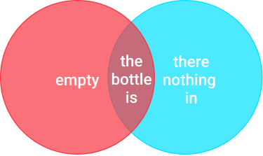
Size of the intersection of the two sets: 3

Size of the union of the two sets: 1+3+3 = 7

Using the Jaccard index, we get a similarity score of 3/7 = 0.42

Python function for Jaccard similarity:

Testing the function for our example sentences

Euclidean Distance

Euclidean distance, or L2 norm, is the most commonly used form of the Minkowski distance. Generally speaking, when people talk about distance, they refer to Euclidean distance. It uses the Pythagoras theorem to calculate the distance between two points as indicated in the figure below:

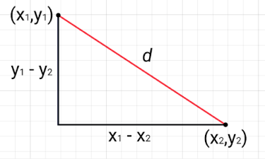
The larger the distance d between two vectors, the lower the similarity score and vice versa. 

Let’s compute the similarity between our example statements using Euclidean distance:

To compute the Euclidean distance we need vectors, so we’ll use spaCy’s in-built Word2Vec model to create text embeddings. (We’ll learn more about this later in the article)

Okay, so we have the Euclidean distance of 1.86, but what does that mean? See, the problem with using distance is that it’s hard to make sense if there is nothing to compare to. The distances can vary from 0 to infinity, we need to use some way to normalize them to the range of 0 to 1.

Although we have our typical normalization formula that uses mean and standard deviation, it is sensitive to outliers. That means if there are a few extremely large distances, every other distance will become smaller as a consequence of the normalization operation. So the best option here is to use something like the Euler’s constant as follows:

Cosine Similarity

Cosine Similarity computes the similarity of two vectors as the cosine of the angle between two vectors. It determines whether two vectors are pointing in roughly the same direction. So if the angle between the vectors is 0 degrees, then the cosine similarity is 1.

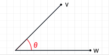
It is given as:

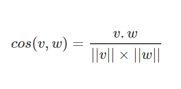
Where ||v|| represents the length of the vector v, 𝜃 denotes the angle between v  and w, and ‘.’ denotes the dot product operator.

What Metric To Use?

Jaccard similarity takes into account only the set of unique words for each text document. This makes it the likely candidate for assessing the similarity of documents when repetition is not an issue. A prime example of such an application is comparing product descriptions. For instance, if a term like “HD” or “thermal efficiency” is used multiple times in one description and just once in another, the Euclidean distance and cosine similarity would drop. On the other hand, if the total number of unique words stays the same, the Jaccard similarity will remain unchanged. 

Both Euclidean and cosine similarity metrics drop if an additional ‘empty’ is added to our first example sentence:

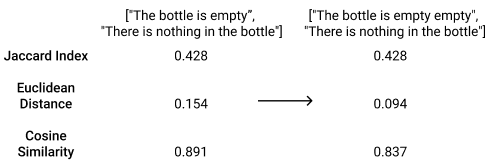
That being said, Jaccard similarity is rarely used when working with text data as it does not work with text embeddings. This means that is limited to assessing the lexical similarity of text, i.e., how similar documents are on a word level.

As far as cosine and Euclidean metrics are concerned, the differentiating factor between the two is that cosine similarity is not affected by the magnitude/length of the feature vectors. Let’s say we are creating a topic tagging algorithm. If a word (e.g. senate) occurs more frequently in document 1 than it does in document 2,  we could assume that document 1 is more related to the topic of Politics. However, it could also be the case that we are working with news articles of different lengths. Then, the word ‘senate’ probably occurred more in document 1 simply because it was way longer. As we saw earlier when the word ‘empty’ was repeated, cosine similarity is less sensitive to a difference in lengths.

In addition to that, Euclidean distance doesn’t work well with the sparse vectors of text embeddings. So cosine similarity is generally preferred over Euclidean distance when working with text data.  The only length-sensitive text similarity use case that comes to mind is plagiarism detection. 

Text Embeddings

Humans can easily understand and derive meaning from words, but computers don’t have this natural neuro-linguistic ability. To make words machine-understandable we need to encode them into a numeric form, so the computer can apply mathematical formulas and operations to make sense of them. Even beyond the task of text similarity, representing documents in the form of numbers and vectors is an active area of study. 

Word Embeddings

Simply put, word embedding is the vector representation of a word. They aim to capture the meaning, context, and semantic relationships of the words. A lot of the word embeddings are created based on the notion of the “distributional hypothesis” introduced by Zellig Harris: words that are used close to one another typically have the same meaning. 

One-Hot Encoding & Bag-of-Words 

The most straightforward way to numerically represent words is through the one-hot encoding method. The idea is simple, create a vector with the size of the total number of unique words in the corpora.  Each unique word has a unique feature and will be represented by a 1 with 0s everywhere else.  

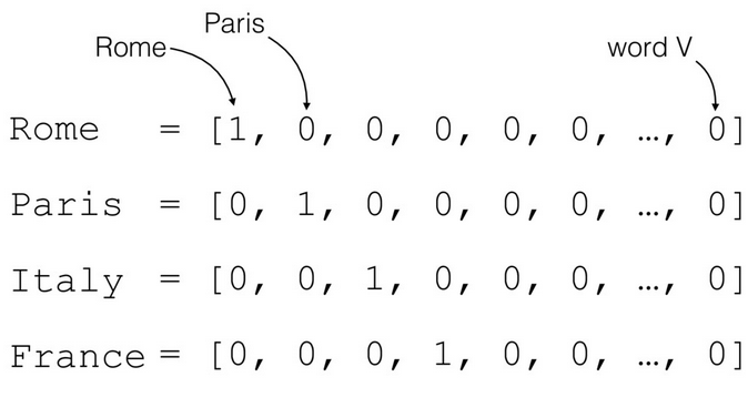
Documents contain large chunks of text with the possibility of repetition. Simply marking the presence or absence of words leads to loss of information.  In the "bag of words" representation (also called count vectorizing), each word is represented by its count instead of 1. Regardless of that, both these approaches create huge, sparse vectors that capture absolutely no relational information.

Implementation

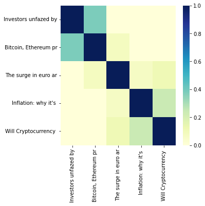
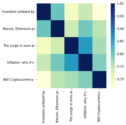
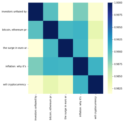
The scikit-learn module implements this method, let’s use it to calculate the similarity of the following news headlines:

To make for better output, let’s create a function that creates a heatmap of the similarity scores.

Now that we have our data and helper function, we can test countvectorizer

Term Frequency-Inverse Document Frequency (TF-IDF)

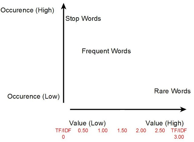
TF-IDF vectors are an extension of the one-hot encoding model. Instead of considering the frequency of words in one document, the frequency of words across the whole corpus is taken into account. The big idea is that words that occur a lot everywhere carry very little meaning or significance. For instance, trivial words like “and”, “or”,  “is” don’t carry as much significance as nouns and proper nouns that occur less frequently.

Mathematically, Term Frequency (TF) is the number of times a word appears in a document divided by the total number of words in the document. And Inverse Document Frequency (IDF) = log(N/n) where N is the total number of documents and n is the number of documents a term has appeared in. The TF-IDF value for a word is the product of the term frequency and the inverse document frequency. 

Although TF-IDF vectors offer a slight improvement over simple count vectorizing, they still have very high dimensionality and don’t capture semantic relationships. 

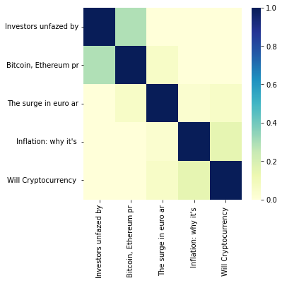
Implementation

Scikit-learn also offers a `TfidfVectorizer` class for creating TF-IDF vectors from the text. 

Word2Vec

Word2Vec is a predictive method for forming word embeddings. Unlike the previous methods that need to be “trained” on the working corpus, Word2Vec is a pre-trained two-layer neural network. It takes as input the text corpus and outputs a set of feature vectors that represent words in that corpus.  It uses one of two neural network-based methods: 

• Continuous Bag Of Words (CBOW)
• Skip-Gram 

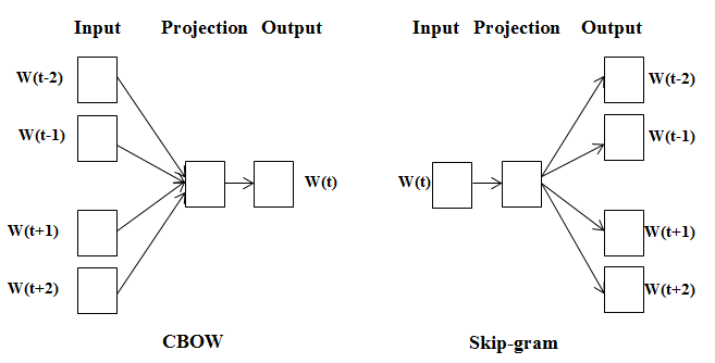
Continuous Bag Of Words takes the context of each word as the input and tries to predict the word corresponding to the context. Here, context simply means the surrounding words. 

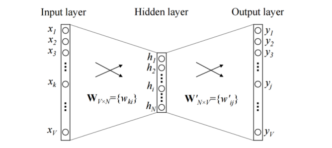
For example, consider the greeting: “Have a nice day”

Let’s say we use the word ‘nice’ as the input to the neural network and we are trying to predict the word ‘day’. We will use the one-hot encoding of the input word ‘nice’, then measure and optimize for the output error of the target word ‘day’.  In this process of trying to predict the target word, this shallow network learns its vector representation.

Just like how this model used a single context word to predict the target, it can be extended to use multiple context words to do the same:

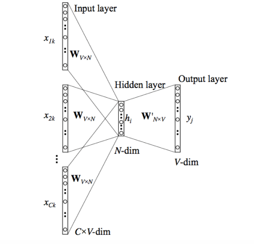
So CBOW generates word representations based on the context words, but there’s another way to do the same. We can use the target word, i.e., the word we want to generate the representation for, to predict the context.

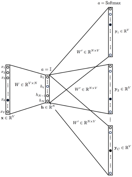
That’s what Skip-gram does. In the process of predicting the context words, the Skip-gram model learns the vector representation of the target word. representations are generated using the context words.

When To Use What? 

Intuitively, the CBOW task is much simpler as it is using multiple inputs to predict one target while Skip-gram relies on one-word inputs. This is reflected in the faster convergence time of  CBOW, in the original paper the authors wrote that CBOW took hours to train, while Skip-gram took 3 days.

Continuing on the same train of thought, CBOW is better at learning syntactic relationships between words while skip-gram is better at understanding the semantic relationships. In practical terms, this means that for a word like ‘dog’, CBOW would return morphologically similar words like plurals like ‘dogs’. On the other hand, Skip-gram would consider morphologically different but semantically similar words like ‘cat’ or ‘hamster’.

And lastly, as Skip-gram relies on single-word input it is less sensitive to overfitting frequent words. Because even if some words appear more times during the training they considered one at a time. CBOW is prone to overfit frequent words because they can appear several times in the same set of context words. This characteristic also allows Skip-gram to be more efficient in terms amount of documents required to achieve good performance. 

TLDR: Skip-gram works better when working with a small amount of data, focuses on semantic similarity of words, and represents rare words well. On the other hand, CBOW is faster,  focuses more on the morphological similarity of words, and needs more data to achieve similar performance.

Implementation

Word2Vec is used in spaCy to create word vectors, one important thing to note: In order to create word vectors we need larger spaCy models. For example, For example, the medium or large English model, but not the small one. So if we want to use vectors, we will go with a model that ends in 'md' or 'lg'. More details about this can be found here.

Install spaCy and download one of the larger models:

Create a pipeline object and use it to create to the Docs for the headlines:

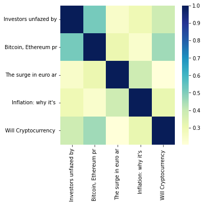
We can look up the embedding vector for the `Doc` or individual tokens using the `.vector` attribute. Let’s see what the headline embeddings look like.

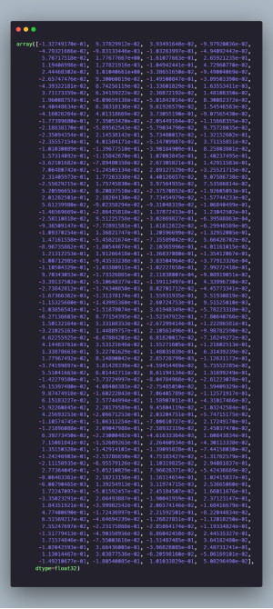
The result is a 300-dimensional vector of the first headline. We can use these vectors to calculate the cosine similarity of the headlines. spaCy `doc` object have their own `similarity` method that calculates the cosine similarity.

Need For Contextual Embeddings

So far all the text embeddings we have covered learn a global word embedding. They first build a vocabulary of all the unique words in the document, then learn similar representations for words that appear together frequently. The issue with such word representations is that the words’ contextual meaning is ignored.  In practice, this approach to word representation does not address polysemy or the coexistence of many possible meanings for a given word or phrase. For instance, consider the following statement :

“After stealing gold from the bank vault, the bank robber was seen fishing on the river bank.”

Traditional word embedding techniques will only learn one representation for the word ‘bank’. But ‘bank’ has two different meanings in the sentence and needs to have two different representations in the embedding space. Contextual embedding methods like BERT and ELMo learn sequence-level semantics by considering the sequence of all words in the document. As a result, these techniques learn different representations for polysemous words like ‘bank’ in the above example, based on their context. 

ELMo

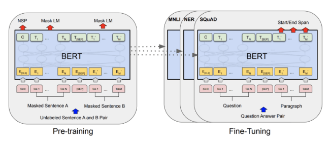
ELMo computes the embeddings from the internal states of a two-layer bidirectional Language Model (LM), thus the name “ELMo”: Embeddings from Language Models. It assigns each word a representation that is a function of the entire corpus of sentences. ELMo embeddings are a function of all of the internal layers of the biLM. Different layers encode different kinds of information for the same word. For example, the lower levels work well for Part-Of-Speech tagging, while the higher levels are better at dealing with polysemous words. 

Concatenating the activations of all layers allows ELMo to combine a wide range of word representations that perform better on downstream tasks. In addition to that, ELMo works on the character level instead of words. This enables it to take advantage of sub-word units to derive meaningful embeddings for even out-of-vocabulary words. 

This means that the way ELMo is used is quite different compared to traditional embedding methods. Instead of having a dictionary of words and their corresponding vectors, ELMo creates embeddings on the fly.

Implementation

There are many implementations of ELMo, we’ll be trying out the simpe-elmo module.  We’ll also need to download a pre-trained model to create the embeddings

Now, let's create an ElmoModel instance and load the pre-trained model we just downloaded.

Create the text embedding

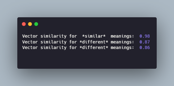
The Tensor’s second dimension of 92 corresponds to the 92 characters in the sentence. To get the word embeddings we can average the embeddings of the characters for each word. Our main concern is ELMo’s ability to extract contextual information so let’s focus only on the three instances of the word “bank”:

We can now evaluate how similar the three instances are:

Sentence Embeddings

So far we have discussed how word embeddings represent the meaning of the words in a text document. But sometimes we need to go a step further and encode the meaning of the whole sentence to readily understand the context in which the words are used. This sentence representation is important for many downstream tasks. It enables us to understand the meaning of the sentence without calculating the individual embeddings of the words. It also allows us to make comparisons on the sentence level. 

Using simple mathematical manipulation, it is possible to adapt sentence embeddings for tasks such as semantic search, clustering, intent detection, paraphrase detection. In addition to that, cross-lingual sentence embedding models can be used for parallel text mining or translation pair detection. For example, the TAUS Data Marketplace uses a data cleaning technique that uses sentence embeddings to compute the semantic similarity between parallel segments of text in different languages to assess translation quality.  

A straightforward approach for creating sentence embeddings is to use a word embedding model to encode all words of the given sentence and take the average of all the word vectors. While this provides a strong baseline, it falls short of capturing information related to word order and other aspects of overall sentence semantics.

Doc2Vec

The Doc2Vec model (or Paragraph Vector) extends the idea of the Word2Vec algorithm. The algorithm follows the assumption that a word’s meaning is given by the words that appear close by. Similar to Word2Vec, Doc2Vec has two variants. 

Distributed Memory Model(DM)

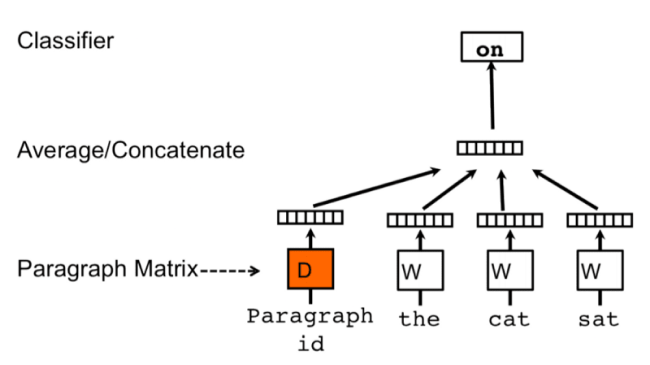
Each word and sentence of the training corpus are one-hot encoded and stored in matrices D and W, respectively. The training process involves passing a sliding window over the sentence, trying to predict the next word based on the previous words and the sentence vector (or Paragraph Matrix in the figure above). This prediction of the next word is done by concatenating the sentence and word vectors and passing the result into a softmax layer. The sentence vectors change with sentences, while the word vectors remain the same. Both are updated during training. 

The inference process also involves the same sliding window approach. The difference is that all the vectors of the models are fixed except the sentence vector. After all the predictions of the next word are computed for a sentence, the sentence embedding is the resultant sentence vector.

Distributed Bag-Of-Words (DBOW) Model

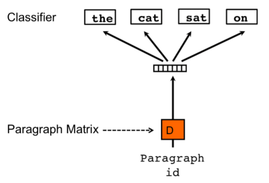
The DBOW model ignores the word order and has a simpler architecture. Each sentence in the training corpus is converted into a one-hot representation. During training, a random sentence is selected from the corpus, and from the sentence, a random number of words. The model tries to predict these words using only the sentence ID, and the sentence vector is updated(Paragraph ID and Paragraph Matrix in the figure).

During inference, a new sentence ID is trained with random words from the sentence. The sentence vector is updated in each step, and the resulting sentence vector is the embedding for that sentence.

What Variant To Use?

The DM model takes into account the word order, the DBOW model doesn’t. Also, the DBOW model doesn’t use word vectors so the semantics of the words are not preserved. As a result, it’s harder for it to detect similarities between words. And because of its simpler architecture, the DBOW model requires more training to obtain accurate vectors. The main drawback of the DM model is the time and the resources needed to generate an embedding, which is higher than with the DBOW model.

What approach produces better Sentence Embeddings? In the original paper, the authors state that the DM model is “consistently better than” DBOW. However, later studies showed that the DBOW approach is better for most tasks. For that reason, the implementation in the Gensim of Doc2Vec uses the DBOW approach as the default algorithm. 

Implementation

Install Gensim,  get the “text8” dataset to train the Doc2Vec model.

Tag the text data, then use it to build the model vocabulary and train the model.

Use the model to get the sentence embeddings of the headlines and calculate the cosine similarity between them.

Sentence Transformers

Much like ELMo, there are a few bidirectional LSTM based sentence encoders (InferSent, etc) but LSTMs have certain problems. Firstly, they use a hidden vector to represent the memory at the current state of the input. But for long input sequences such as sentences, a single vector isn't enough to provide all the information needed to predict the next state correctly. This bottleneck of the size of the hidden vector makes LSTM based methods more susceptible to mistakes, as in practice it can only hold information from a limited number of steps back. The Attention mechanism in transformers doesn’t have this bottleneck issue as it has access to all the previous hidden states for making predictions. 

Another problem with LSTMs is the time to train. As the output is always dependent on the previous input, the training is done sequentially. This makes parallelization harder and results in longer training times. The Transformer architecture parallelized the use of the Attention mechanism in a neural network allowing for lower training time. 

Transformer-based general language understanding models perform much better than all their predecessors. When BERT was introduced, it achieved state-of-the-art results in a wide range of tasks such as question answering or language inference with minor tweaks in its architecture. That being said, it has a massive computational overhead. For example, finding the most similar pair of sentences in a collection of 10,000 requires about 50 million inference computations (~65 hours). The structure of BERT makes it unsuitable for semantic similarity search as well as for unsupervised tasks like clustering. 

Sentence-BERT (SBERT) is a modified BERT network that uses siamese and triplet network structures to derive semantically meaningful sentence embeddings. This reduces the effort for finding the most similar pair from 65 hours with BERT / RoBERTa to about 5 seconds with SBERT, while maintaining the accuracy from BERT. 

Implementation

We’ll try out the RoBERTa based models implemented in the sentence-transformer module.

Download the 'stsb-roberta-large' model.

Use it to calculate the headline embeddings and their pairwise similarity.

Universal Sentence Encoder

Google’s Universal Sentence Encoder(USE) leverages a one-to-many multi-tasking learning framework to learn a universal sentence embedding by switching between several tasks. The 6 tasks, skip-thoughts prediction of the next/previous sentence, neural machine translation, constituency parsing, and natural language inference, share the same sentence embedding. This reduces training time greatly while preserving the performance on a variety of transfer tasks.

One version of the Universal Sentence Encoder model uses a deep average network (DAN) encoder, while another version uses a Transformer.

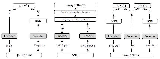
The more complicated Transformer architecture performs better than the simpler DAN model on a variety of sentiment and similarity classification tasks. The compute time for the Transformer version increases noticeably as sentence length increases. On the other hand, the compute time for the DAN model stays nearly constant as sentence length increases.

Implementation

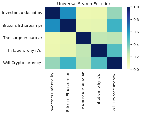
What Embedding To Use?

As a general rule of thumb, traditional embeddings techniques like Word2Vec and Doc2Vec offer good results when the task only requires the global meaning of the text. This is reflected in their outperformance of state-of-the-art deep learning techniques on tasks such as semantic text similarity or paraphrase detection. On the other hand, when the task needs somethings more specific than just the global meaning, take for example sentiment analysis or sequence labeling, more complex contextual methods perform better.

So always start with a simple and fast method as the baseline before moving on to more complex methods if required.